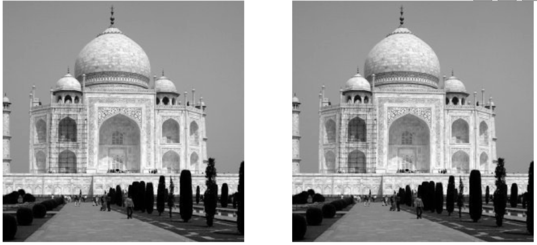
Original and Reconstructed Taj Image
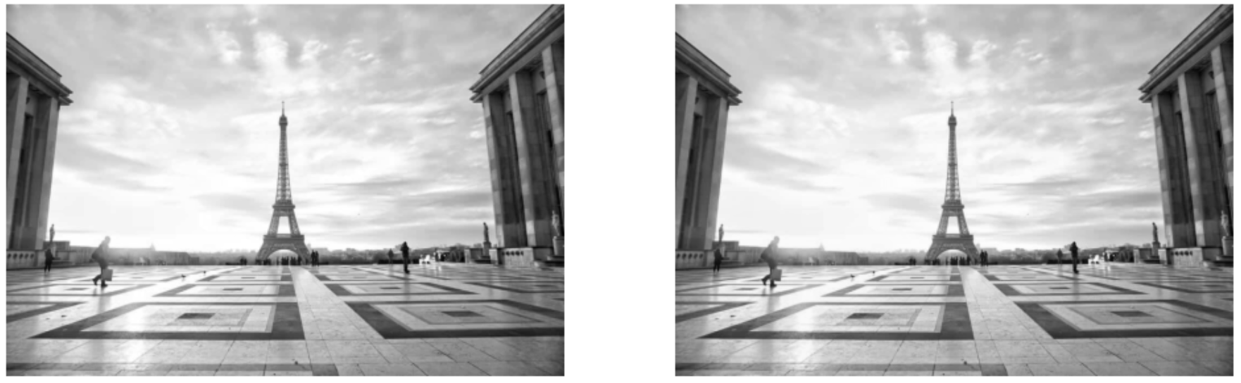
Original and Reconstructed Paris Image
This part explores gradient-domain processing, a technique used for applications like blending. The primary focus is on "Poisson blending," a method to seamlessly blend an object or texture from a source image into a target image without visible seams. This provides an alterative to using than Gaussian and Laplacian Pyramids.
In this part, I solve a toy problem to reconstruct an image using its x and y gradients and a single pixel value.
This section demonstrates gradient-domain processing by reconstructing an image from its gradients and a single known pixel value.
The goal is to ensure the implementation is correct before applying it to more complex tasks.
First I define objectives to match x and y gradients of the source image while anchoring one pixel's intensity.
I formulate the problem as a least squares optimization: min ||Av - b||^2, where:
A: Encodes gradient and intensity constraints.
v: Unknown pixel values to solve.
b: Gradient differences and fixed intensity.
Then, I solve for v using a least squares solver and map the result to reconstruct the image.
Below is an example of a reconstructed image compared to the original which appear the same as it was recovered correctly.
Original and Reconstructed Taj Image
Original and Reconstructed Paris Image
The goal of Poisson blending is to seamlessly blend a source region into a target image.
This is achieved by solving a set of blending constraints as a least squares optimization problem.
First, I define the region in the source image and its placement in the target image and
align the regions.
Then I use a least squares optimization to ensure gradient continuity between the source and target regions and
copy the solved pixel values into the target image.
For each pixel \( i \) in the source region, I
minimize (v_i - v_j - (s_i - s_j))^2
where \( j \) is a neighboring pixel. This ensures the gradient between \( i \) and \( j \)
in the blended region matches the source image. If a pixel \( j \) is in the target region, the constraint becomes:
minimize (v_i - t_j - (s_i - s_j))^2
where \( t_j \) is the intensity from the target image. I combine all of these constraints into a sparse matrix equation:
A * v = b
where \( A \) encodes the constraints, \( v \) is the vector of unknown intensities, and \( b \) contains the gradient differences and fixed intensities.
For RGB images, I process each color channel separately.
Below are examples of successful blends and a couple of failure cases. Failure cases were mainly caused by
large differences in lighting of the source and target images.
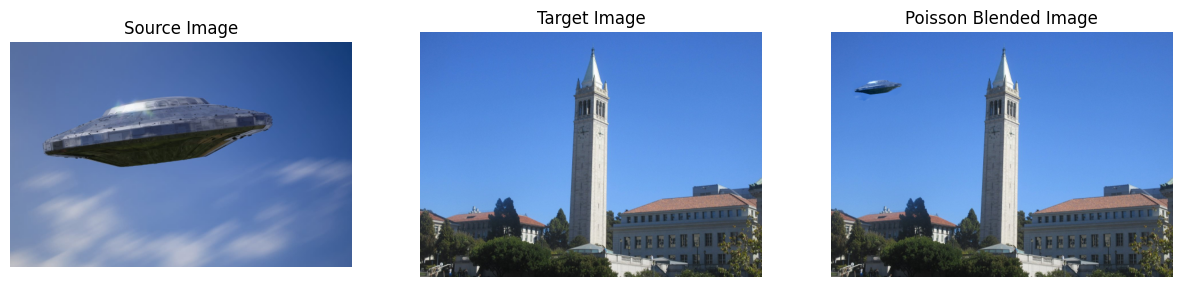
UFO blended into the UC Berkeley Sky.
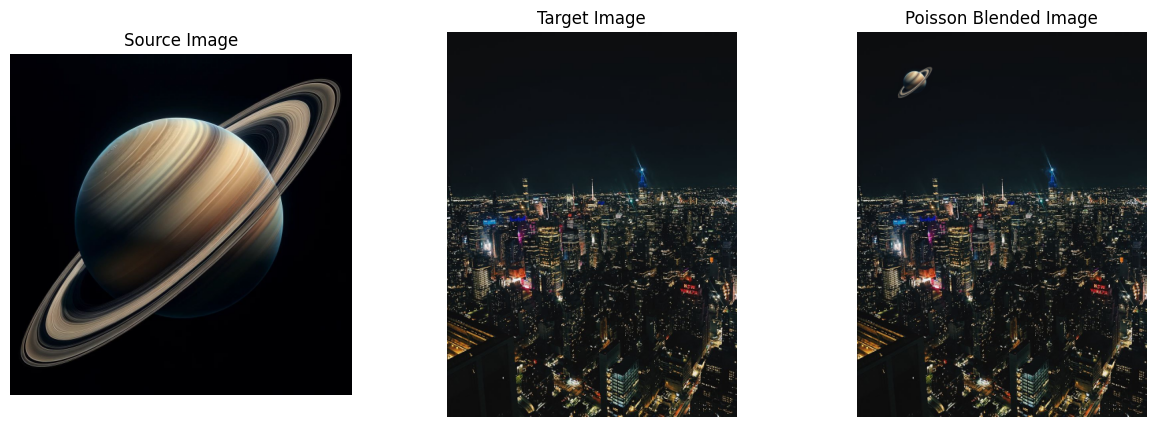
Saturn blended into the New York Skyline.
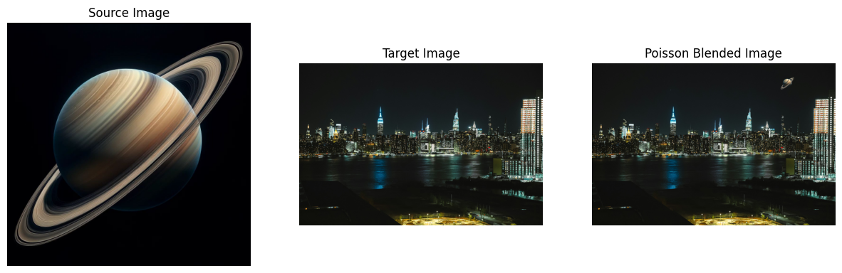
Saturn blended into another New York Skyline.
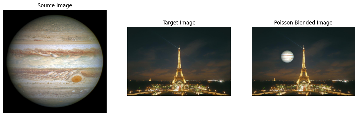
Jupiter blended next to the Eifel Tower.
Mask used for UFO blending.
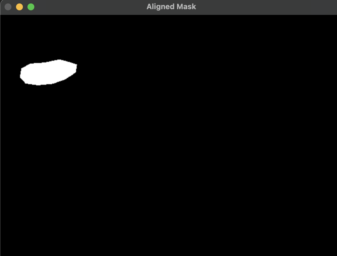
Masked used for Saturn blending into the New York Skyline.
Masked used for Saturn blending into another New York Skyline.
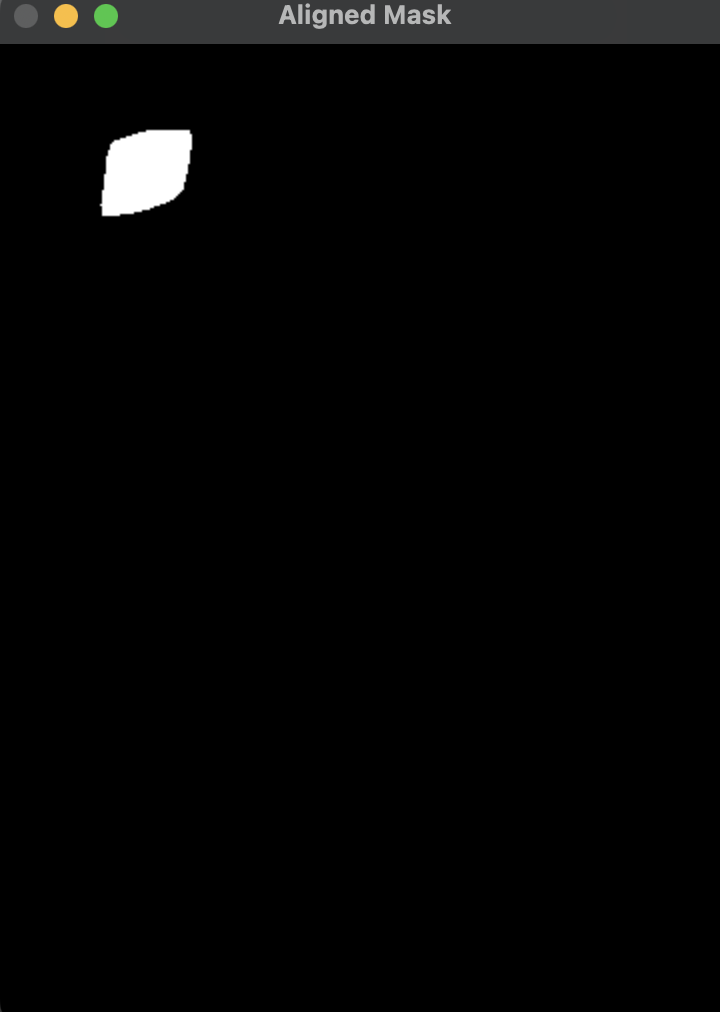
Masked used for Jupiter blending next to the Eifel Tower.
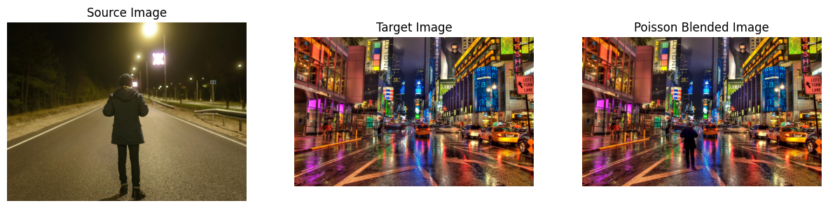
Suboptimal results for blending a man into New York stree due to large lighting differences.
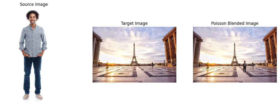
Suboptimal results for blending a man onto Paris street due to lighting differences.
Mixed gradients use the larger gradient magnitude from either the source or target image. This technique helps preserve stronger details from both images. Below is an example using mixed gradients for blending some writing onto a wall.
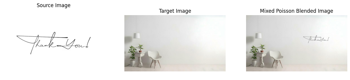
Mixed Gradient Blending of text onto a wall.
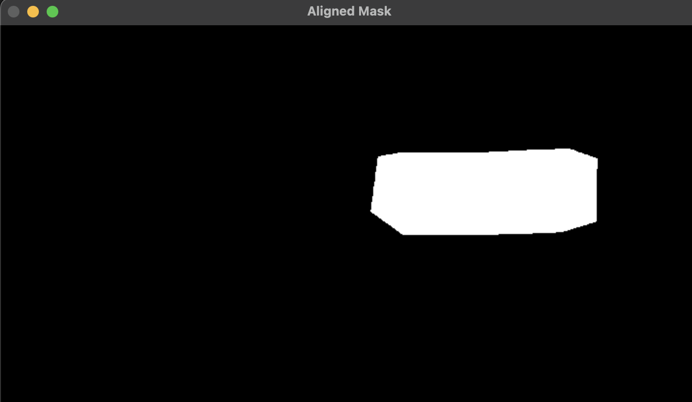
Mixed Gradient Blending mask of text onto a wall.
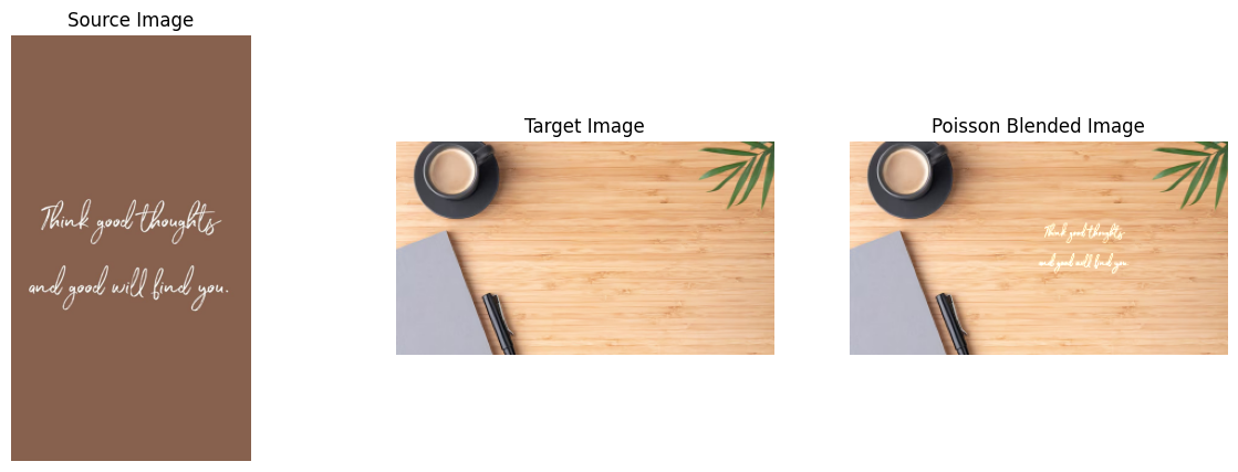
Mixed Gradient Blending of text onto a desk.
This project explores the effects achievable using lightfield data, such as depth refocusing and aperture adjustment. I use a dataset of a chess board to show how shifting and averaging multiple images can achieve visual effects of depth focus and different apertures.
Objects farther from the camera remain stationary across images in the lightfield grid, while closer objects shift significantly. Averaging all images without shifting focuses on distant objects, while appropriate shifts focus on nearer objects. If all images are averaged without applying any shifts, the resulting image will appear sharp for distant objects but blurry for closer ones. By adjusting the shifts at various scales before averaging, we can bring objects at different depths into focus. Below is a GIF of images focused at different depths.
Depth refocusing gif.
Depth refocusing gif with more frames.
Combining a large set of images sampled across a grid perpendicular to the optical axis simulates the effect of a camera with a larger aperture. Conversely, using fewer images creates a result resembling a smaller aperture. By varying the selection radius for the images utilizing a L1 distance metric, I can produce results corresponding to different aperture sizes while maintaining focus on the same point. By averaging a larger subset of lightfield images, we simulate a larger aperture, resulting in a shallower depth of field. Using fewer images simulates a smaller aperture. Below is a GIF of images captured with different simulated aperture sizes for a fixed focus point.
Aperture gif with C=0.5
Aperture gif with C = 0.4
This project demonstrates the versatility of lightfield data in generating complex visual effects using simple operations. This project also signifies the simplicity of creating these affects as all that is requried is simply averaging and shifting the images within the dataset. Techniques like depth refocusing and aperture adjustment highlight the potential of lightfield cameras for computational photography.